Unit Hydrograph Methods
Overview
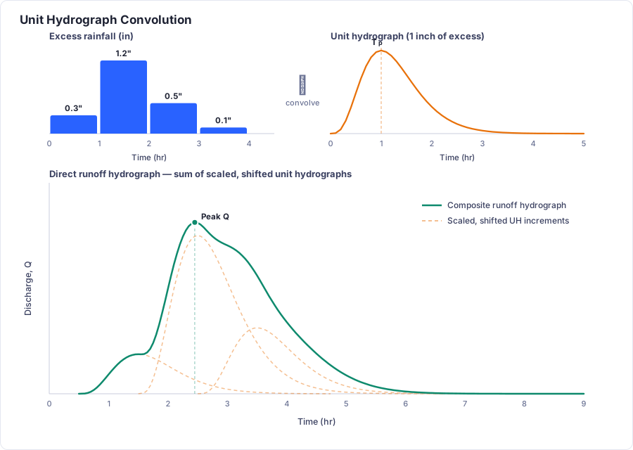
A unit hydrograph (UH) is the direct runoff hydrograph resulting from one inch of excess rainfall applied uniformly over a basin for a specified duration. The actual runoff hydrograph for any storm is computed by convolving the excess rainfall with the unit hydrograph, a process that distributes each rainfall increment's contribution across time and sums them.
The Convolution Process
- Compute excess rainfall (rainfall minus losses) for each time step
- For each excess rainfall increment, scale the unit hydrograph by that increment
- Shift each scaled hydrograph by the appropriate time step
- Sum all the shifted, scaled hydrographs to produce the total direct runoff hydrograph
Transform Methods
HydraLink currently uses the SCS Curvilinear unit hydrograph as its transform method. Additional transform methods (Clark, Snyder, ModClark) are planned for future releases.
SCS Curvilinear
The SCS (now NRCS) curvilinear unit hydrograph is widely used for ungauged watersheds.
Key Equations
where D = computational time step. Use a step no larger than about 0.29 × tlag (HEC-HMS guidance); HydraLink warns when it is larger, since a coarse step flattens the unit-hydrograph peak.
where A = area (mi²), default Peaking Factor = 484 cfs·hr/mi². The dimensionless hydrograph shape is defined by the SCS curvilinear ordinates.
The peak rate factor is set per basin in the basin panel (or the quick-edit grid); Project Settings sets the default applied to new basins. Lower values (284 for coastal plain, 256 or 100 for very flat terrain) produce a flatter, broader hydrograph; 600 models steep, flashy response.
Peak Rate Factor
The Peak Rate Factor (PRF) controls how sharply the unit hydrograph peaks for a given basin area and time to peak. The standard SCS value is 484, which reflects average watershed conditions. Flatter, low-relief watersheds (coastal areas, for example) are often modeled with a lower PRF, around 284, producing a flatter, more delayed hydrograph, while steeper mountainous watersheds may call for a higher PRF than the standard value. Set the project default in Project Settings and override it per basin when local design criteria call for it. A PRF of 484 uses the standard SCS curvilinear dimensionless unit hydrograph; other values reshape the curve per NEH-630.
Planned Transform Methods
The following transform methods are planned for future releases but are not currently active in HydraLink:
Clark (Planned)
The Clark method separates translation (time-area curve) and attenuation (linear reservoir). Parameters include Tc, storage coefficient R, and a time-area curve.
Snyder (Planned)
The Snyder method is an empirical approach based on observed hydrographs from gauged watersheds. Parameters include peaking coefficient Cp and standard lag time tp.
ModClark (Planned)
A variant of the Clark method with modified time-area processing.
Transform Method Summary
| Method | Calibration Needed | Best For | Parameters |
|---|---|---|---|
| SCS | None | Ungauged small-to-medium watersheds | Tc only (lag derived) |
| Clark (planned) | — | Separate control of translation and attenuation | Tc, R |
| Snyder (planned) | — | Gauged watersheds with observed data | Cp, tp |
| ModClark (planned) | — | Modified Clark with improved time-area resolution | Tc, R |
References
- NRCS (2010). National Engineering Handbook, Part 630, Chapter 16, Hydrographs.
- Clark, C.O. (1945). "Storage and the Unit Hydrograph." Transactions, ASCE.
- Snyder, F.F. (1938). "Synthetic Unit-graphs." Transactions, AGU.
- USACE (2000). Hydrologic Modeling System HEC-HMS Technical Reference Manual.