Storm Events

Overview

Storm events define the rainfall input for your HydraLink model. Each storm event specifies a return period, total rainfall depth, duration, and rainfall distribution. HydraLink supports multiple storm types to cover different design scenarios and regional requirements.

Storm Event Parameters

Parameter	Units	Description
Name	—	User-defined storm label (e.g., “100-yr, 24-hr”)
Return Period	years	Design storm recurrence interval (e.g., 2, 5, 10, 25, 50, 100)
Total Rainfall Depth	inches	Total precipitation over the storm duration
Storm Duration	hours	Duration of the storm (default 24 hours)
Storm Distribution	—	Temporal distribution of rainfall within the storm
K Factor	—	Frequency adjustment factor (default 1.0)

Storm Distributions

SCS Rainfall Distributions

The NRCS (formerly SCS) developed four standard 24-hour rainfall distributions based on regional rainfall patterns across the United States:

Distribution	Region	Peak Intensity Timing	Description
Type I	Pacific maritime (CA, OR, WA coast)	~10 hours	Gentle, drawn-out storms
Type IA	Pacific Northwest inland	~8 hours	Least intense of all types
Type II	Central and Eastern US (most common)	~12 hours	Moderate intensity with sharp peak
Type III	Gulf Coast and Atlantic tropical	~12 hours	Highest intensity, tropical storms

Each distribution defines the cumulative fraction of total rainfall at each time increment across the 24-hour storm. The distributions are defined at 6-minute (0.1-hour) intervals (241 data points) and use cubic spline interpolation for sub-interval accuracy.

Custom Distribution

Define your own temporal rainfall pattern. Enter cumulative rainfall fractions at user-specified time intervals. This allows modeling of:

• Non-standard storm durations
• Historical observed storm patterns
• Local design storms mandated by specific jurisdictions

Frequency Storm (Alternating Block Method)

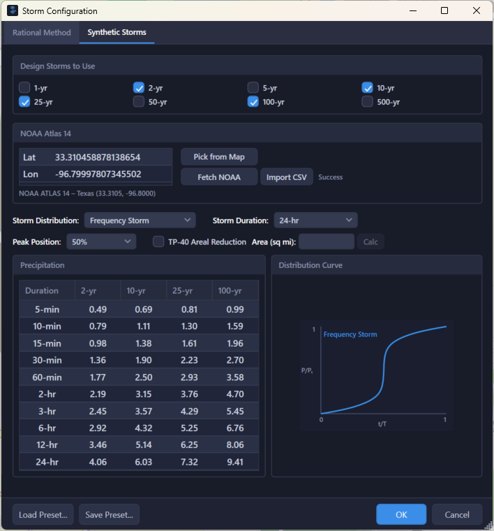
The Frequency Storm uses NOAA Atlas 14 precipitation frequency data to construct a design storm using the HEC-HMS alternating block method:

1. Retrieve depth-duration-frequency data from NOAA Atlas 14 for the project location
2. Compute incremental depths for each duration interval
3. Sort incremental blocks in descending order
4. Alternate placement: highest block at center, then alternating left and right
5. The result is a symmetric storm with peak intensity at the center

This method produces a storm that matches the IDF curve at every duration simultaneously — meaning the storm is the design storm for all sub-durations, not just the 24-hour duration.

NOAA Atlas 14 Precipitation Data

HydraLink integrates with NOAA Atlas 14 to retrieve precipitation frequency estimates for any location in the United States.

What NOAA Atlas 14 Provides

• Precipitation depths for multiple durations (5-minute through 60-day)
• Multiple return periods (1-year through 1000-year)
• Confidence intervals (90% upper and lower bounds)
• Point precipitation estimates based on regional frequency analysis

How to Use in HydraLink

1. Open the Storm Events dialog
2. Click the NOAA Atlas 14 lookup button
3. Enter your project coordinates (latitude/longitude) or click on the map
4. HydraLink retrieves and stores the full precipitation frequency dataset
5. Individual storm events can then reference this data for their total rainfall depth

Common Return Periods

Return Period	Typical Application
2-year	Water quality treatment, minor drainage
5-year	Minor storm sewer design
10-year	Storm sewer design, minor road crossings
25-year	Major storm sewer, roadway drainage
50-year	Major crossings, critical infrastructure
100-year	Floodplain management, detention design, major structures
500-year	Dam safety, emergency spillways

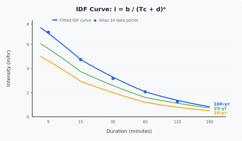
IDF Curve Coefficients (E, B, D)

The IDF (Intensity-Duration-Frequency) curve is central to the Rational Method and Modified Rational Method. It defines how rainfall intensity varies with storm duration for a given return period.

IDF Equation

Where:

• i = rainfall intensity (in/hr)
• T_c = duration (minutes)
• b = numerator parameter
• d = time shift parameter (minutes)
• e = exponent parameter (dimensionless)

Sources of E, B, D Coefficients

HydraLink provides multiple ways to obtain IDF coefficients:

1. Manual Entry of E, B, D Values

You can directly enter E, B, D (or e, b, d) values from published IDF tables, local drainage manuals, or jurisdictional standards (e.g., TxDOT Hydraulic Design Manual tables). This is useful when your jurisdiction provides pre-computed coefficients for the project location.

2. Import NOAA Atlas 14 Values

HydraLink can import NOAA Atlas 14 precipitation frequency data by entering the project coordinates (latitude/longitude). Atlas 14 provides rainfall depths for a comprehensive matrix of durations (5-minute through 60-day) and return periods (1-year through 1000-year). This data serves as the basis for IDF curve fitting.

3. Develop E, B, D from NOAA Atlas 14 (Curve Fitting)

Once Atlas 14 data is imported, HydraLink performs a least-squares optimization to fit the E, B, D coefficients to the depth-duration-frequency data for each return period. The fit quality is reported as:

• R² — Coefficient of determination (goodness of fit)
• Max % Error — Maximum percent deviation between the fitted curve and the Atlas 14 data points

This allows the engineer to evaluate whether the fitted IDF curve adequately represents the Atlas 14 data for the project location.

4. Develop E, B, D from User-Entered Intensity Data

You can also enter intensity-duration data points manually (from local rainfall studies, gauge records, or other sources) and have HydraLink fit the E, B, D coefficients to your custom data. This is useful when working with non-NOAA rainfall sources or site-specific rainfall records.

Atlas 14 Interpolation Modes

When using NOAA Atlas 14 data directly (without IDF curve fitting), HydraLink must interpolate between the discrete duration data points to determine rainfall depth or intensity at any arbitrary duration. Two interpolation modes are available:

Log-Log Interpolation (Default)

Performs interpolation in log-transformed space (both duration and depth are log-transformed before interpolation). This produces a more accurate curve fit of Atlas 14 data because depth-duration-frequency relationships are approximately linear on a log-log scale. Log-log interpolation generally provides better results, particularly for shorter durations where the intensity curve has more curvature.

Linear Interpolation

Performs standard linear interpolation between adjacent Atlas 14 data points in arithmetic space. While simpler, this may not follow the natural curvature of the DDF relationship as closely as log-log interpolation, especially between widely spaced duration intervals.

How Rainfall Intensity is Resolved

For the Rational Method and Modified Rational Method, HydraLink resolves rainfall intensity using the following priority order:

1. IDF Curve Coefficients (e, b, d) — If IDF coefficients exist for the return period (either auto-fitted from NOAA Atlas 14 intensity data or entered manually), the IDF equation i = b / (Tc + d)^e is evaluated at T_c. This takes highest priority.
2. NOAA Atlas 14 Direct Interpolation — If IDF coefficients are not available but Atlas 14 data is loaded, intensity is interpolated directly from the NOAA Atlas 14 intensity-duration-frequency data (log-log or linear interpolation).
3. Fallback — Total storm depth / storm duration. This is a rough approximation and should be avoided for final design.

Additional Uses of IDF Data

• Frequency Storm construction — The IDF data provides the depth-duration relationship used by the alternating block method to build the design hyetograph for Unit Hydrograph analysis.
• Modified Rational Method — MRM detention sizing iterates over multiple storm durations, evaluating the IDF curve at each duration to determine the critical storage requirement.

Synthetic Storm Options for Unit Hydrograph Basins

When using the Unit Hydrograph methodology, a temporal rainfall distribution defines how the total storm depth is distributed over the storm duration. HydraLink provides several synthetic storm options:

SCS Type Distributions

The NRCS (formerly SCS) developed four standard 24-hour dimensionless rainfall distributions. These distributions define the cumulative fraction of total rainfall at each time increment. They are defined at 6-minute (0.1-hour) intervals (241 data points) with cubic spline interpolation for sub-interval accuracy:

Distribution	General Region	Characteristics
Type I	Pacific maritime (CA, OR, WA coast)	Gentle, drawn-out storms with peak at ~10 hours
Type IA	Pacific Northwest inland	Least intense distribution, peak at ~8 hours
Type II	Central and Eastern US	Moderate intensity with sharp peak at ~12 hours
Type III	Gulf Coast and Atlantic tropical	Highest intensity, tropical storms, peak at ~12 hours

The appropriate distribution depends on the project location and local jurisdictional requirements. The engineer should verify which distribution is required for their area.

Frequency Storm (Alternating Block Method)

The Frequency Storm constructs a design storm using the HEC-HMS alternating block method from NOAA Atlas 14 depth-duration-frequency data:

1. Retrieve depths for multiple durations from the Atlas 14 data for the project location
2. Compute incremental depth blocks for each duration interval
3. Sort blocks in descending order of intensity
4. Alternate placement around the storm center: highest block at center, then alternating left and right

The result is a symmetric storm that matches the IDF curve at every sub-duration. This means the storm is simultaneously the design storm for all durations, not just the overall storm duration. This property can be particularly useful for detention design.

Custom Distribution

Define your own temporal rainfall pattern by entering cumulative rainfall fractions at user-specified time intervals. Custom distributions allow modeling of:

• Non-standard storm durations (other than 24 hours)
• Historical observed storm patterns
• Local design storms mandated by specific jurisdictions
• Agency-specific distributions not included in the standard SCS types

Custom distributions must start at (0, 0) and end at (1, 1), with strictly increasing cumulative fractions.

K Factor (Frequency Adjustment)

The K factor allows jurisdictions to apply a safety or frequency adjustment to computed flows. The adjusted Rational Method equation becomes:

Default K = 1.0 (no adjustment). Some jurisdictions (e.g., Dallas County per iSWM Eq 2.20) require K > 1.0 for higher return periods.

Design Storm Selection Guide

Design Objective	Available Approach
Peak flow only (Rational Method)	IDF curve from NOAA Atlas 14 fitting, manual E/B/D entry, or direct Atlas 14 interpolation
Full hydrograph (Unit Hydrograph)	SCS Type distribution, Frequency Storm, or custom distribution
Detention sizing (critical duration)	Frequency Storm (alternating block) captures the critical intensity at all sub-durations
Jurisdictional compliance	Match local requirements for distribution type and rainfall source
Multiple return periods	Create separate storm events for each return period (e.g., 2, 5, 10, 25, 100-yr)

Tips & Best Practices

• Always use NOAA Atlas 14 for the most current precipitation frequency estimates. Older IDF references may be outdated.
• Create multiple storm events (e.g., 2-yr through 100-yr) to evaluate your system across a range of conditions.
• For detention design, include the storm(s) required by your jurisdiction — typically the 100-year event.
• The Frequency Storm is the most conservative approach for detention because it maximizes intensity at every duration.
• Verify that your total rainfall depth matches published values. NOAA Atlas 14 reports depths at the project point, not an areal average.
• For large watersheds (> 10 mi²), consider applying an areal reduction factor to the point rainfall depth.

References

• NOAA (2013). NOAA Atlas 14: Precipitation-Frequency Atlas of the United States.
• NRCS (1986). Urban Hydrology for Small Watersheds, TR-55.
• USACE (2000). HEC-HMS Technical Reference Manual.
• Hershfield, D.M. (1961). Rainfall Frequency Atlas of the United States, TP-40 (superseded by Atlas 14).